You’ve cracked the first step with data – you can tell if its continuous or discrete. As you progress to stats nirvana, you need to delve more deeply into the stuff.

Discrete data (only in certain categories) can be thought of as either ordered, or unordered. Ordered data has values which can be ‘ranked’ somehow – like cancer stage, weight categories, or Apgar score. Unordered data doesn’t have a ‘flow’ to it; eye colour, gender, subspeciality of doctor.

The ordinal (ordered) nature of some discrete data can lead you to do some sorts of testing that you can’t do with unordered (categorical) data.

Continuous data is sometimes Normal, and sometimes it’s not Normal. (I guess we don’t really need to use a capital N, but I tend to use it to put the point across that this is a special Normal not normal normal.)

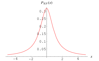
Normally distributed data has a bell shaped distribution (that is, when you plot frequency against value). Data that does not have this shape is ‘non-Normally distributed’. This again has importance – you can do some tests with Normal data that give a more efficient answer than you can with non-Normal data.

We’ll go into means, deviation and other things that sound a little S&M (including correction and transformation) in a future post.

– Archi

(p.s. – please do tag / tweet your favourite thing to be addressed in this series to us when you can)